Building a Neural Network for Regression

5.7. Building a Neural Network for Regression#

We can use sklearn’s MLPRegressor to build a neural network. The letters MLP stand for multilayer perceptron, which is another name for the neural networks we have been looking at.

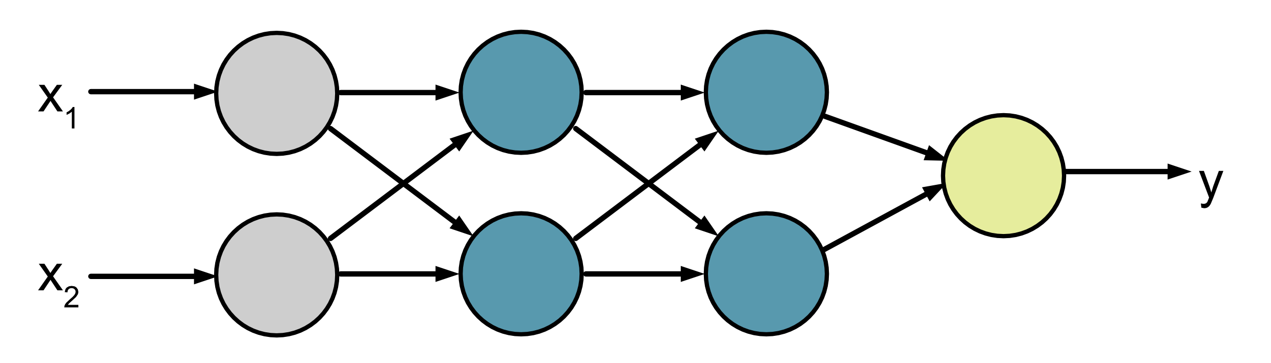
For this example we’ll build a very simple neural network that takes in two inputs \(x_1\) and \(x_2\) and predicts \(y\), where \(y=x_1 + x_2\).

This is the data we’ll be using. sum.csv

from sklearn.neural_network import MLPRegressor
import pandas as pd

data = pd.read_csv("sum.csv")
print(data)

To build our neural network, we import it with the following:

from sklearn.neural_network import MLPRegressor

Then we create an MLPRegressor model.

nn = MLPRegressor(
    hidden_layer_sizes=(2, 2), max_iter=5000, learning_rate_init=0.01, random_state=0
)

Let’s quickly try to understand what each of these arguments mean.

hidden_layer_sizes: This is a tuple that tells you how many neurons are in each hidden layer of the network. In this case (2, 2) means there are 2 neurons in the first hidden layer and then 2 neurons in the second hidden layer. Note that we don’t need to specify the number of neurons in the input and output layer because that can automatically be worked out by the x and y values we provide in .fit() (see below). In this case we feed in two x inputs and we calculate one y output. This means that our neural network will look like this:

max_iter: This sets the maximum number of iterations the neural network will train for.
learning_rate_init: This sets the initial learning rate use for training.
random_state: The initial state, i.e. the value of the weights and biases, will be random. This sets the seed value for the random number generation.

We then fit our model using:

nn.fit(x, y)

And make predictions using:

nn.predict(x)

Here is a short example:

from sklearn.neural_network import MLPRegressor
import pandas as pd
import numpy as np

data = pd.read_csv("sum.csv")
x = data[["x1", "x2"]].to_numpy()
y = data["y"].to_numpy()

nn = MLPRegressor(
    hidden_layer_sizes=(2, 2), max_iter=5000, learning_rate_init=0.01, random_state=0
)
nn.fit(x, y)
pred = nn.predict(x)

x_test = np.array([[-8, -10], [7, 9], [9, -2], [5, -10], [-3, -1]])
print(nn.predict(x_test))

You can see that our model does reasonably well on the test data provided.

\(x_1\)	\(x_2\)	Actual \(y\)	Predicted \(y\) (2 d.p)
-8	-10	-18	-16.99
7	9	16	16.00
9	-2	7	7.00
5	-10	-5	-5.00
-3	-1	-4	-4.00

5.7.1. Visualising Learning#

The following code plots the error of the neural network on the training data for each iteration. We have added one additional argument which is n_iter_no_change=5000. n_iter_no_change can be used to terminate the neural network training early if there is no change in the performance of the neural network for some set number of iterations, i.e. the weights and biases have stopped changing and the neural network has converged. For visualisation purposes we want our network to keep training for 5000 iterations, so we set this to 5000.

For convenience we’ve also suppressed warnings using:

import warnings

warnings.filterwarnings("ignore")

Without it you will get warnings if your neural network hasn’t converged.

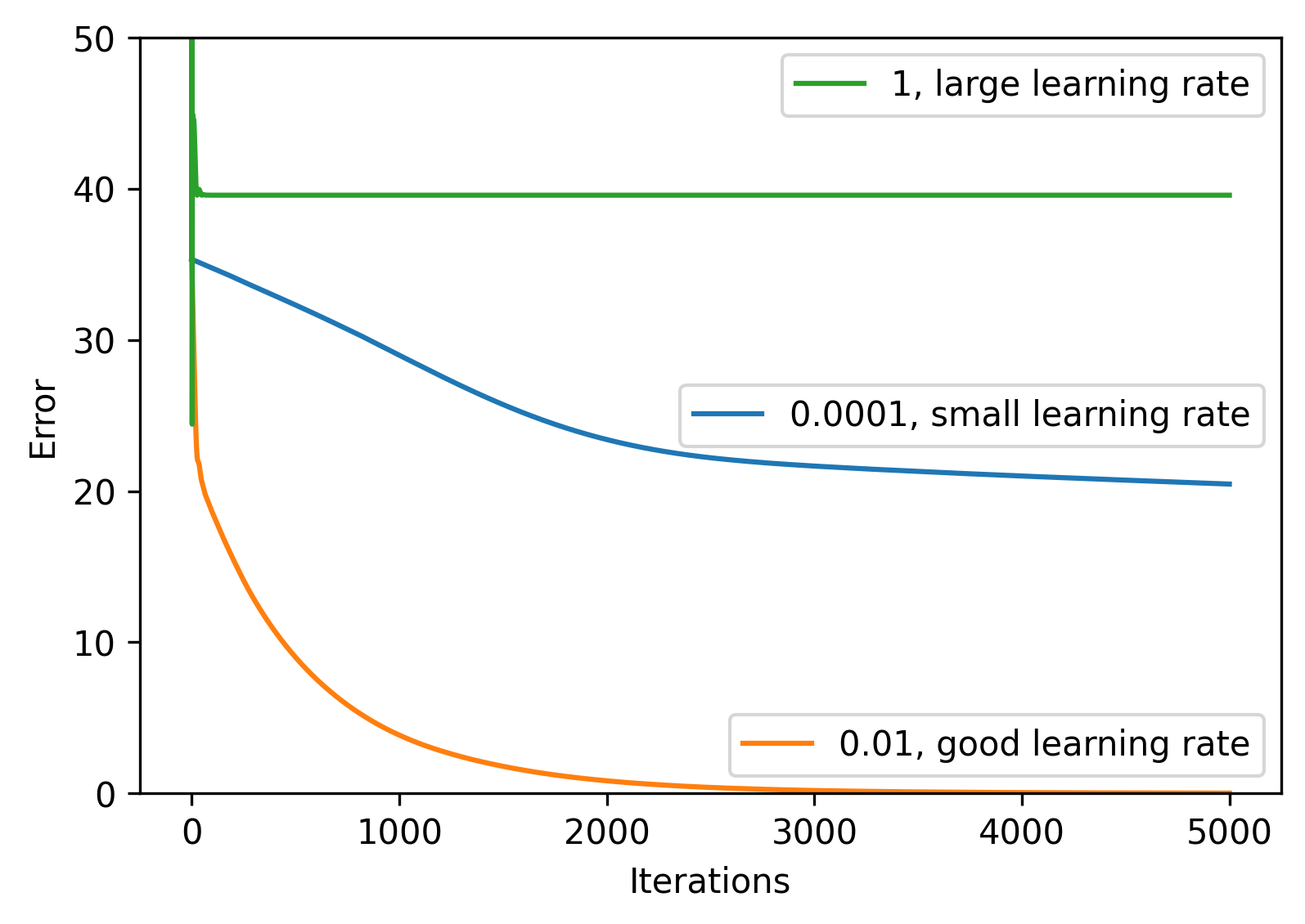
Experiment with changing the learning rate in the code below. sum.csv

from sklearn.neural_network import MLPRegressor
from sklearn.metrics import mean_squared_error as mse
import matplotlib.pyplot as plt
import pandas as pd

import warnings

warnings.filterwarnings("ignore")

data = pd.read_csv("sum.csv")
x = data[["x1", "x2"]].to_numpy()
y = data["y"].to_numpy()

nn = MLPRegressor(
    hidden_layer_sizes=(2, 2),
    max_iter=5000,
    learning_rate_init=0.01,
    random_state=0,
    n_iter_no_change=5000,
)
nn.fit(x, y)

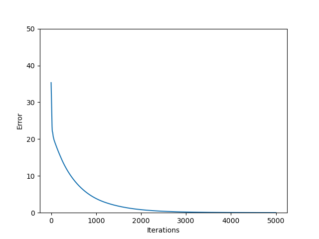
plt.plot(nn.loss_curve_)
plt.ylim([0, 50])
plt.xlabel("Iterations")
plt.ylabel("Error")
plt.savefig("plot.png")

Challenge: Neural Network for Regression

You have been provided with a csv file called rgb_train.csv. This data contains the following columns:

red
green
blue
hue
saturation

Use this data to build a neural network to predict the hue and saturation from the given red, green and blue values.

Instructions

Using pandas, read the file rgb_train.csv into a DataFrame
Extract the 'red', 'green' and 'blue' columns into the variable x
Extract the 'hue' and 'saturation' columns into the variable y
Convert both x and y to numpy arrays
Using sklearn.neural_network, create a MLPRegressor
- The neural network should have 3 hidden layers with 2, 3 and 2 neurons in these layers
- Set the maximum number of iterations to 2000
- Set the learning rate to 0.0002
- Set random_state to 0
Fit the data neural network to the training data
Use the model to make a prediction for the following test samples and print the results.

Sample	Actual
(150, 25, 150)	(300, 71)
(50, 60, 180)	(235, 57)
(250, 200, 170)	(23, 89)

Your output should look like this:

[[XXX.XXXXXXX   XX.XXXXXXXX]
[XXX.XXXXXXXX  XX.XXXXXXXX]
[ XX.XXXXXXXX  XX.XXXXXXXX]]

Building a Neural Network for Regression

Contents

5.7. Building a Neural Network for Regression#

5.7.1. Visualising Learning#