2.2. Polynomial Regression#
Linear regression models fit lines to data.
Polynomial regression extends the capabilities of linear regression in that polynomial regression models fit polynomials to data.
Polynomial regression is:
A form of supervised learning (data is labelled)
A regression algorithm (predict a number)
Polynomials are functions where terms in the equation are raised to a power. The highest power is called the degree of the polynomial. For example
\(y = \beta_0 + \beta_1 x\) is a polynomial of degree 1, since the terms with the highest degree is \(x^1\). This polynomial looks like a line.
\(y = \beta_0 + \beta_1 x + \beta_2 x^2\) is a polynomial of degree 2, since the term with the highest degree is \(x^2\). This polynomial is a parabola.
\(y = \beta_0 + \beta_1 x + \beta_2 x^2 + \beta_3 x^3\) is a polynomial of degree 3, since the term with the highest degree is \(x^3\). This polynomial is a cubic, which looks like an ‘S’.
Polynomials take the general form
where \(p\) is the degree of the polynomial. The polynomial degree can be arbitrarily large. Typically as the polynomial degree increases, the number of ‘wiggles’ in the function increases.
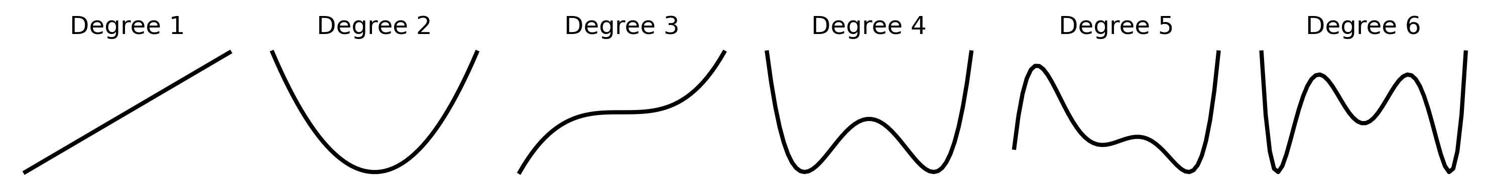
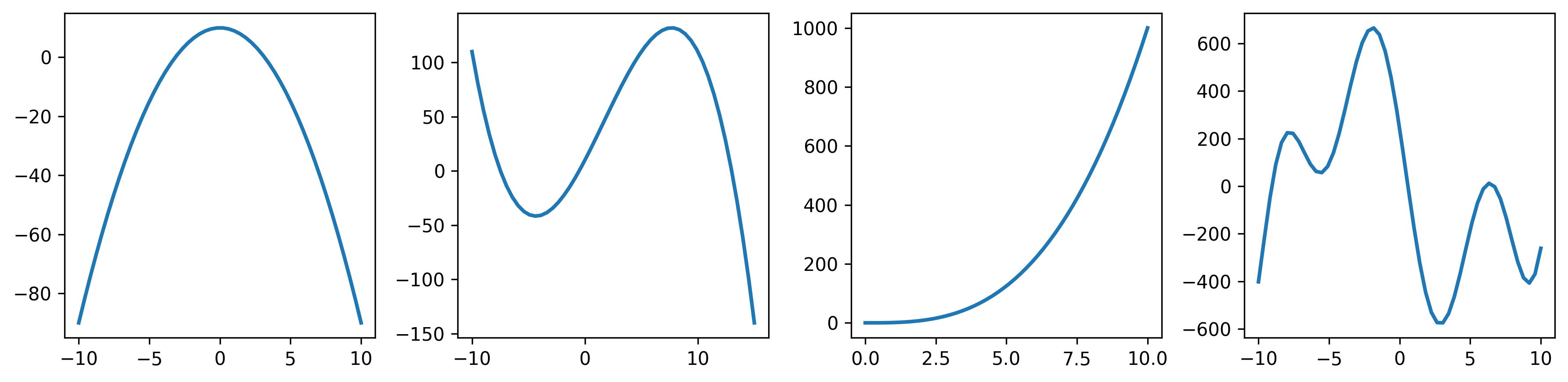
Here are some examples of curves that can be constructed with polynomial functions.
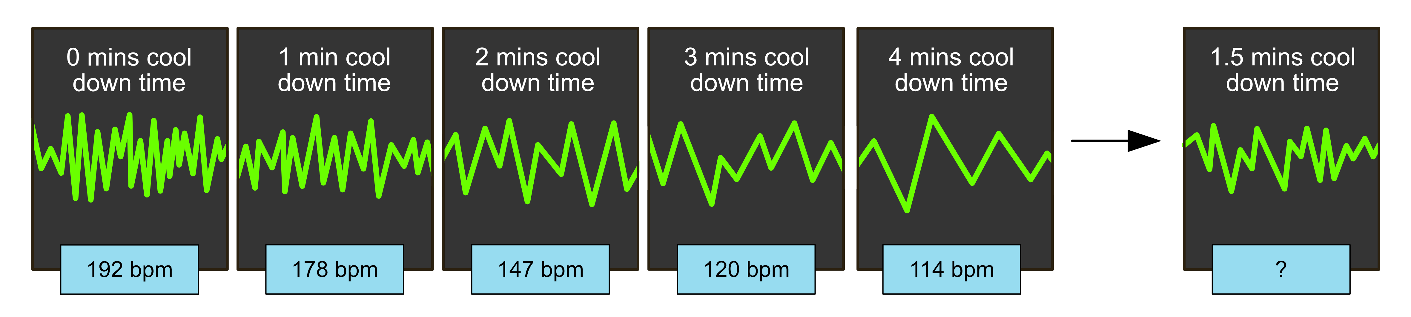
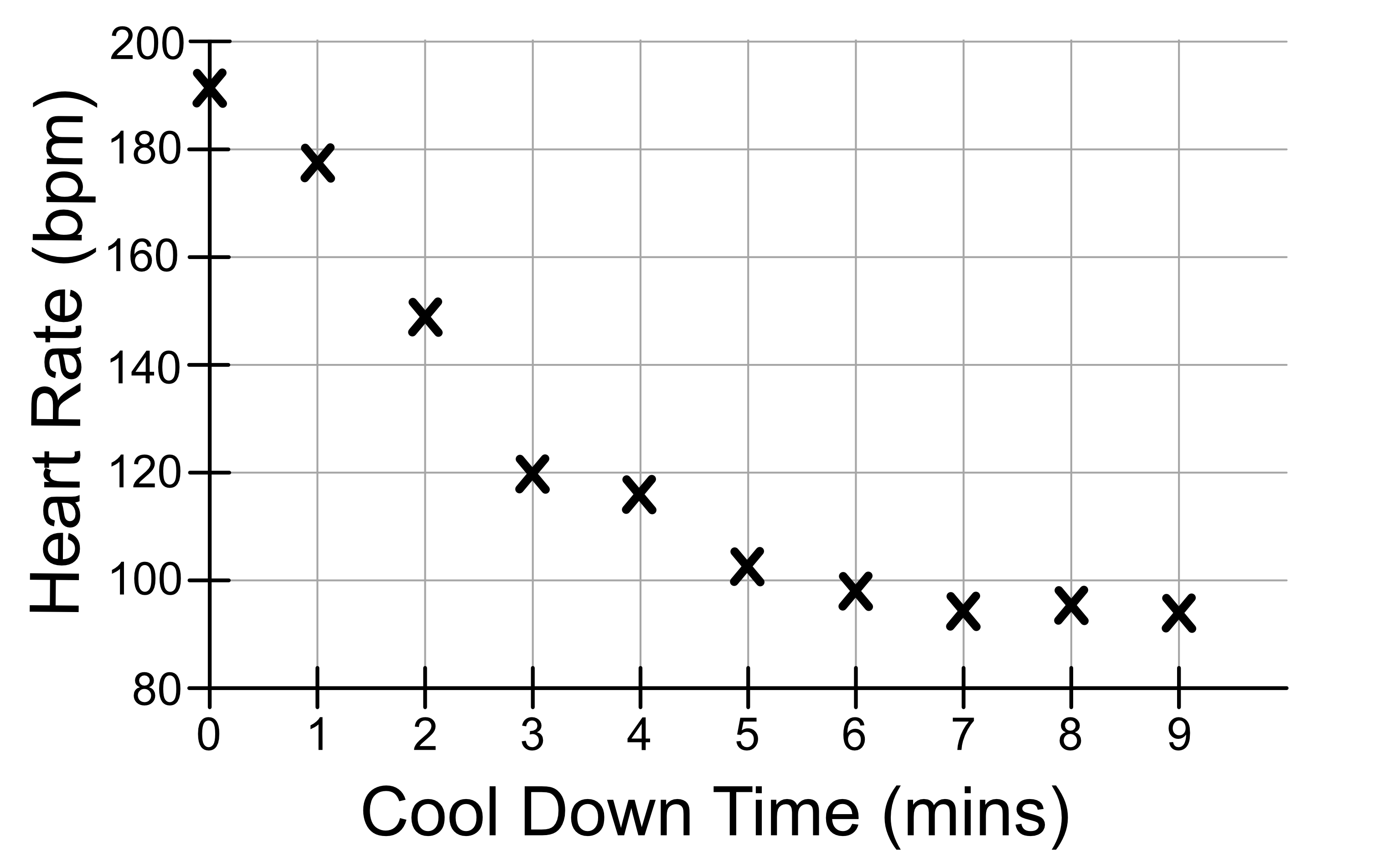
Consider the following dataset:
Heart Rate (bpm) |
Cool Down Time (mins) |
|---|---|
192 |
0 |
178 |
1 |
147 |
2 |
120 |
3 |
114 |
4 |
103 |
5 |
99 |
6 |
93 |
7 |
94 |
8 |
92 |
9 |
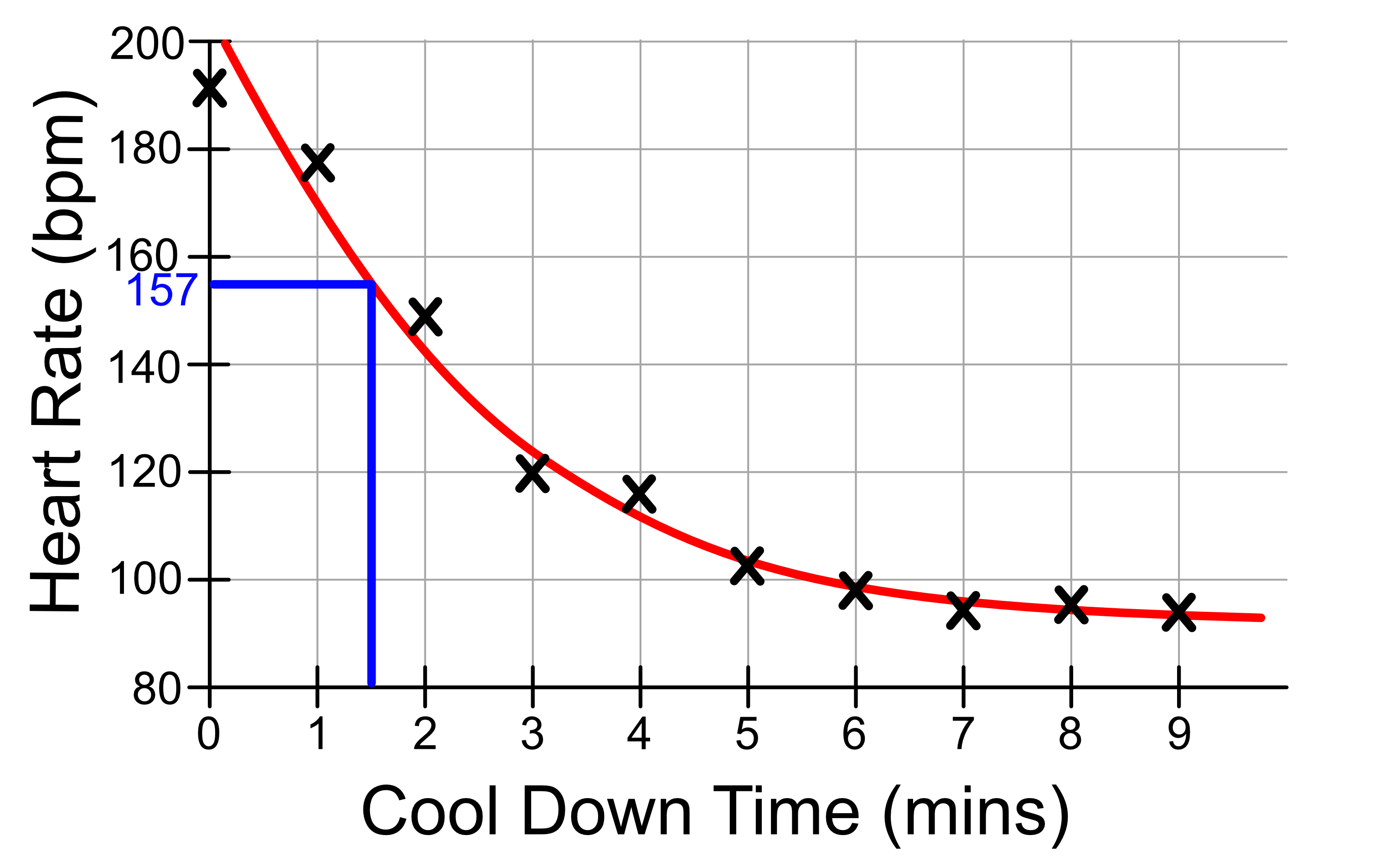
This is what the data looks like on a graph.
With polynomial regression, we aren’t restricted to fitting lines to the data, we are able to fit a curve to it. Our curve might look like this:
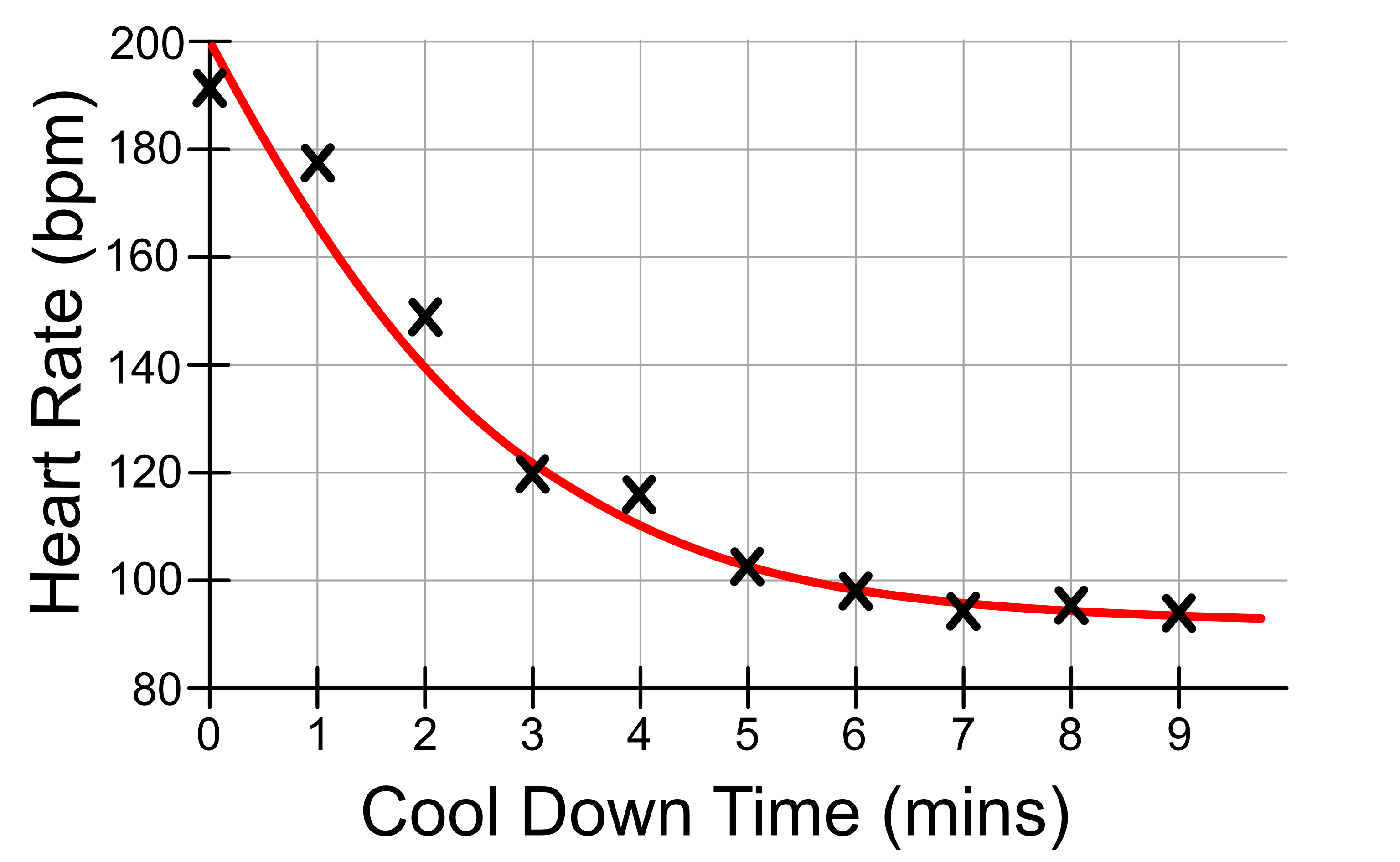
We can use this to predict the heart rate of the athlete at a given cool down time. For example, after 1.5 minutes of cool down, we expect the athlete to have a heart rate of 157 bpm