5.4. Information Flow: Making a Prediction#
So how does a neural network work?
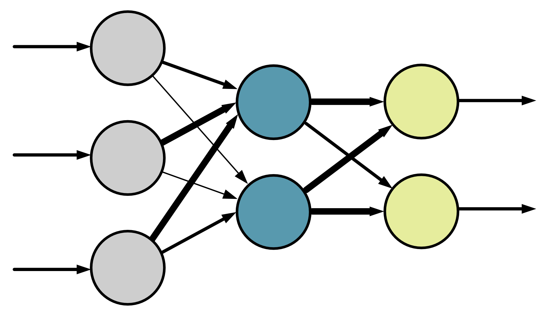
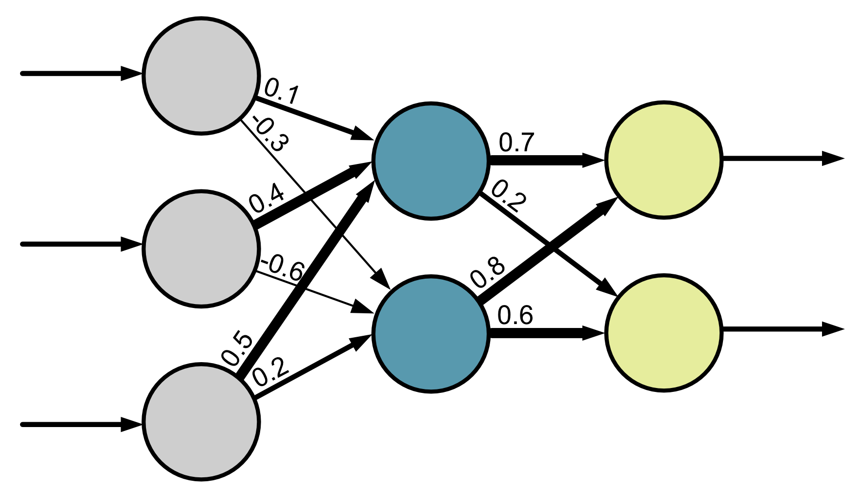
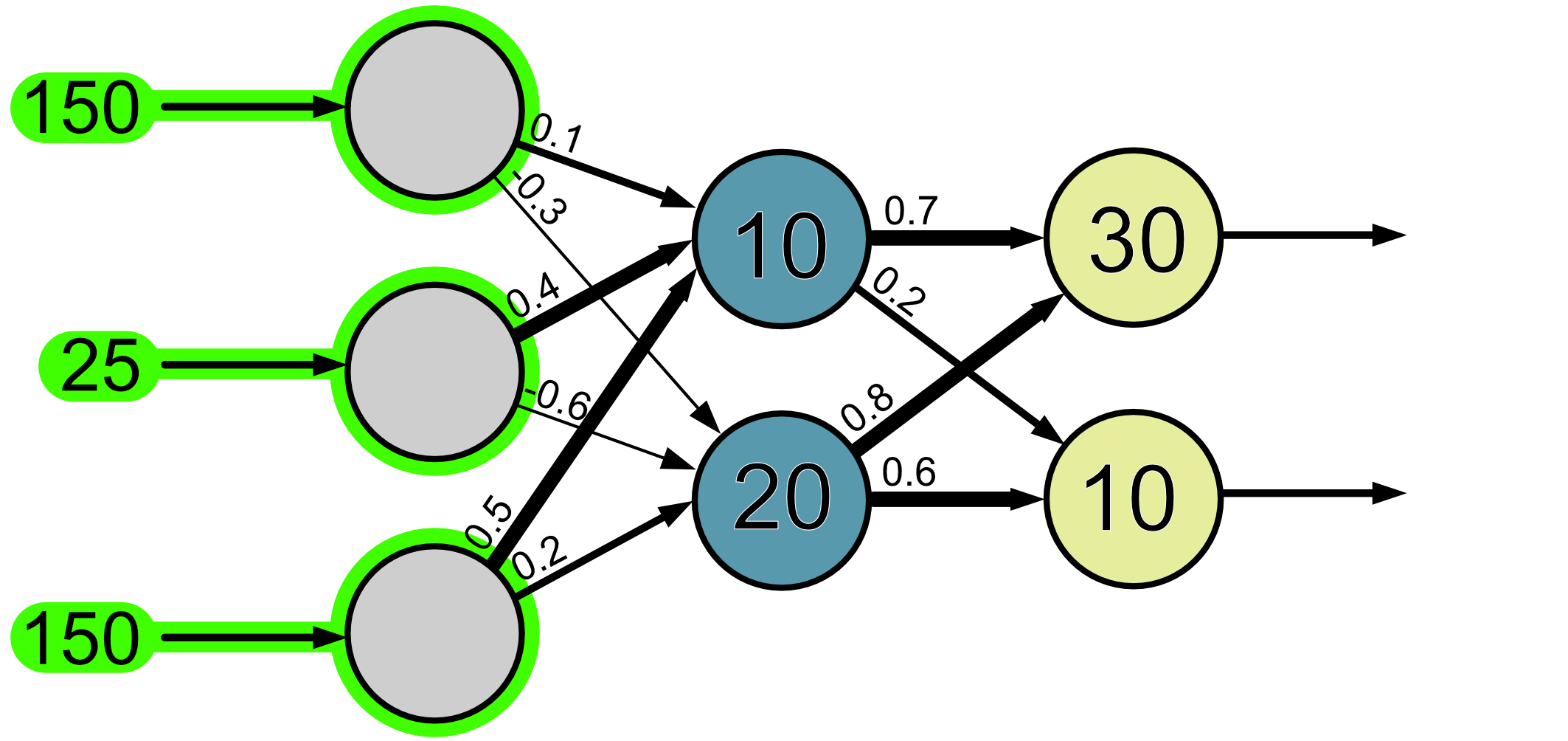
In the brain the neurons are connected in complex networks and these connections, or pathways can be of different strengths. To mimic this in our artificial neural network we assign connections weights. The bigger the weight the stronger the connection. We only care about the weights between neurons. Consider the figure below. For visualisation we have changed the thickness of the connections to reflect the weights.
To represent the weights of each connection in a computer, we use numbers. The value of the number corresponds to the weight of the connection.
Each neuron is also a little bit different. We associate each neuron with a number called a neural network bias, which affects the behaviour of the neuron. We only have a bias for the neurons in the hidden layer and the output layer.
The weights and biases are the model parameters.
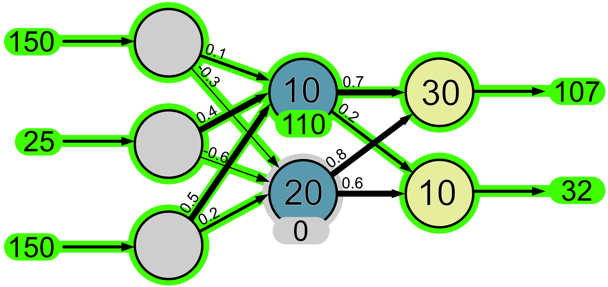
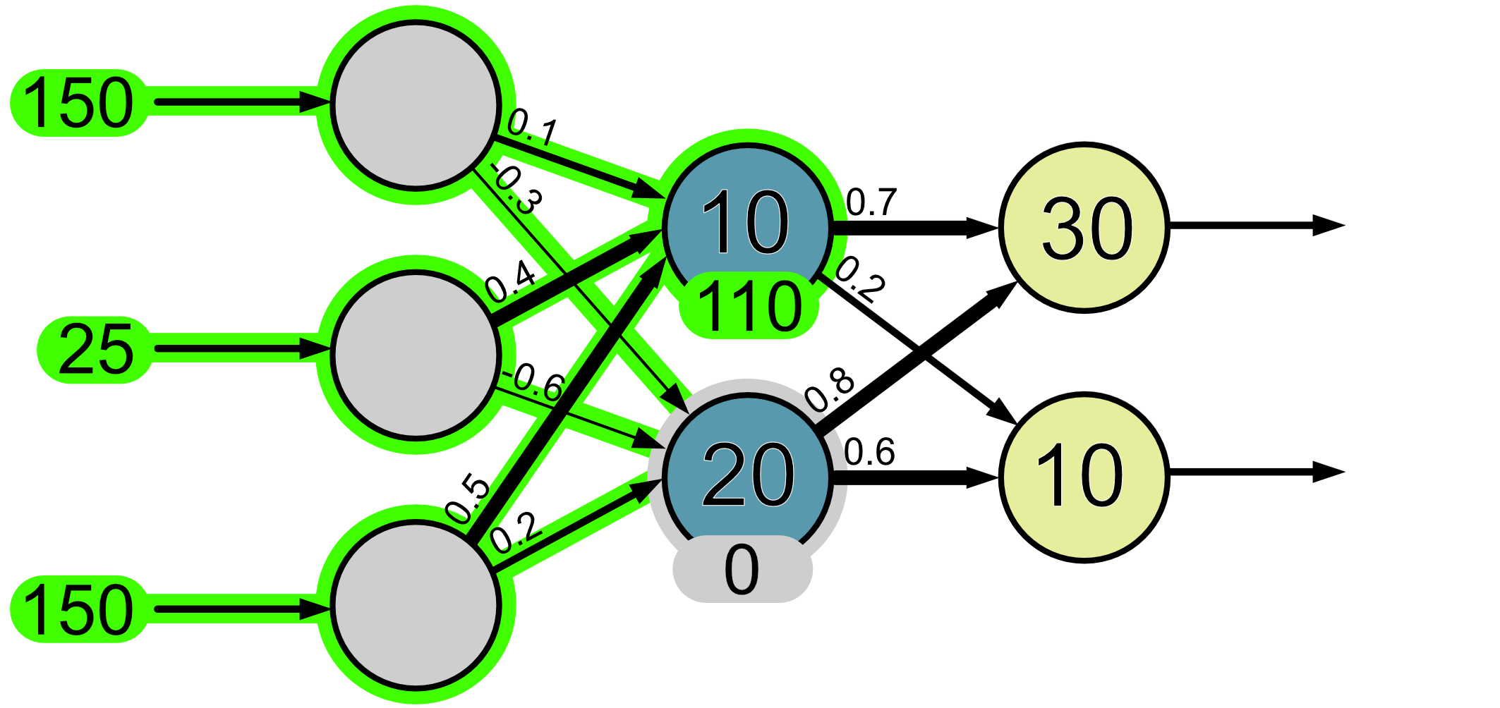
When we input information into our neural network, this information ‘flows’ through the network as a series of mathematical operations. Let’s give our network the input values 150, 25 and 150 and we’ll see step-by-step how they ‘flow’ through the network.
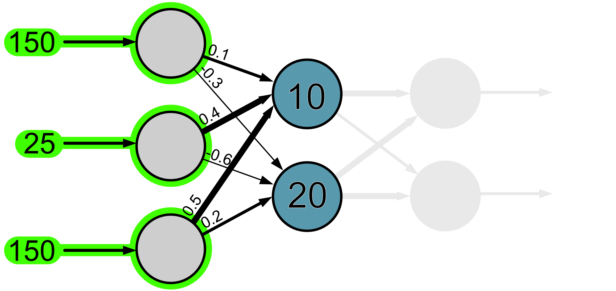
First, the input values make it to the input neurons.
Next, we look at the neurons in the first layer. Since the information flows in the diagram from left to right, we don’t have to worry about anything to the right of these neurons.
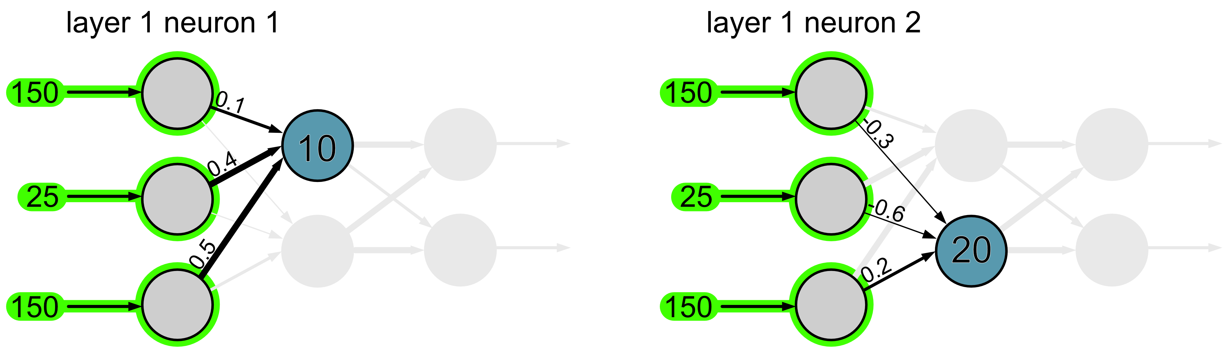
Then to make things easier we’ll look at each neuron separately.
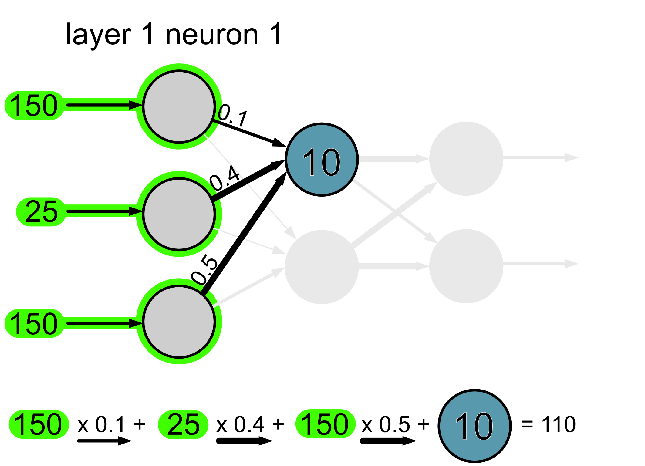
We take the information that is flowing into the neural network and we multiply it by the weights of the connections. So for example if the weight is 1, the full value from that neuron goes through, if the weight is 0.5, half of the value goes through and if the weight is 0, none of it goes through. Then, once all the values arrive at the neuron we add them together and we also add the bias.
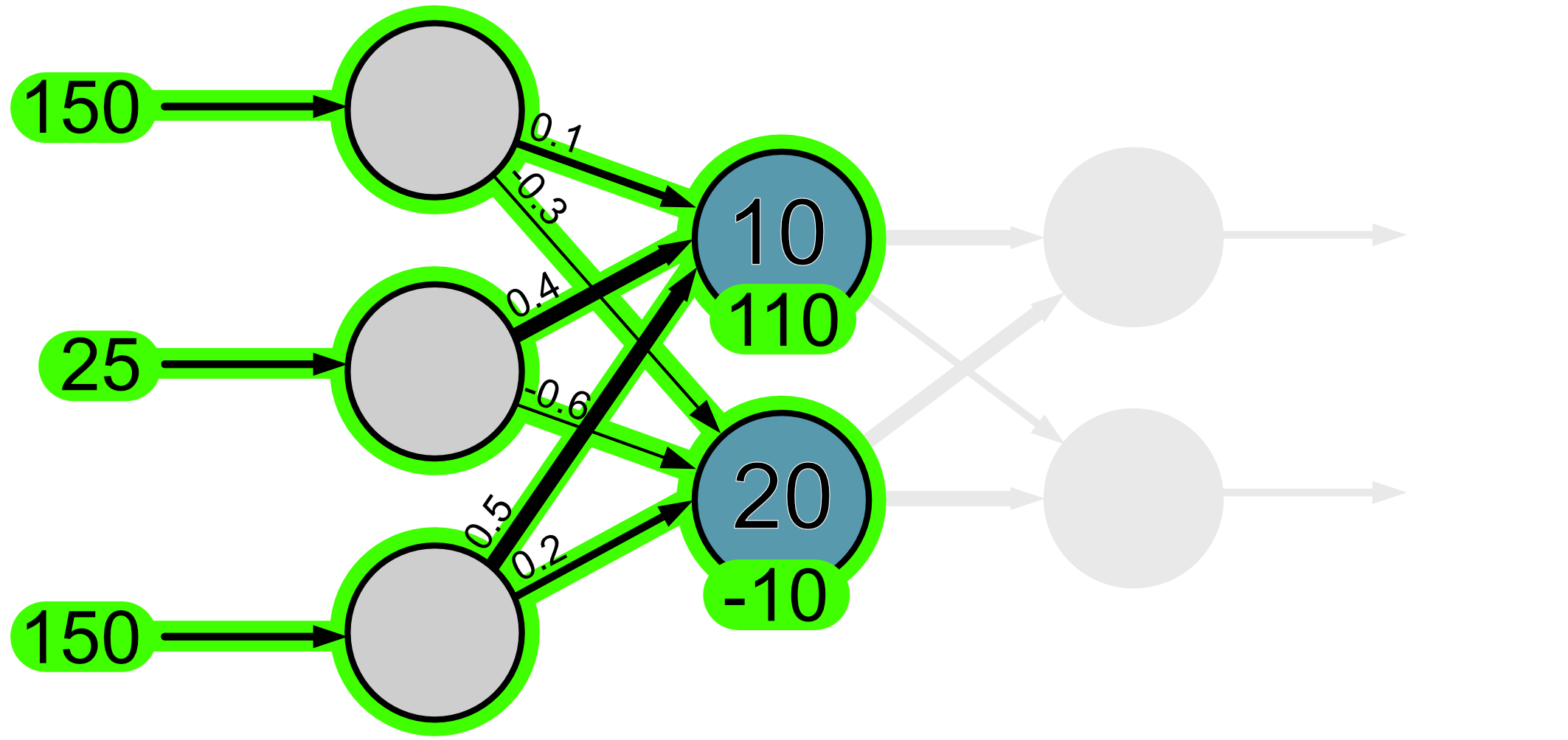
Here’s the calculation for neuron 1.
And here’s the calculation for neuron 2.
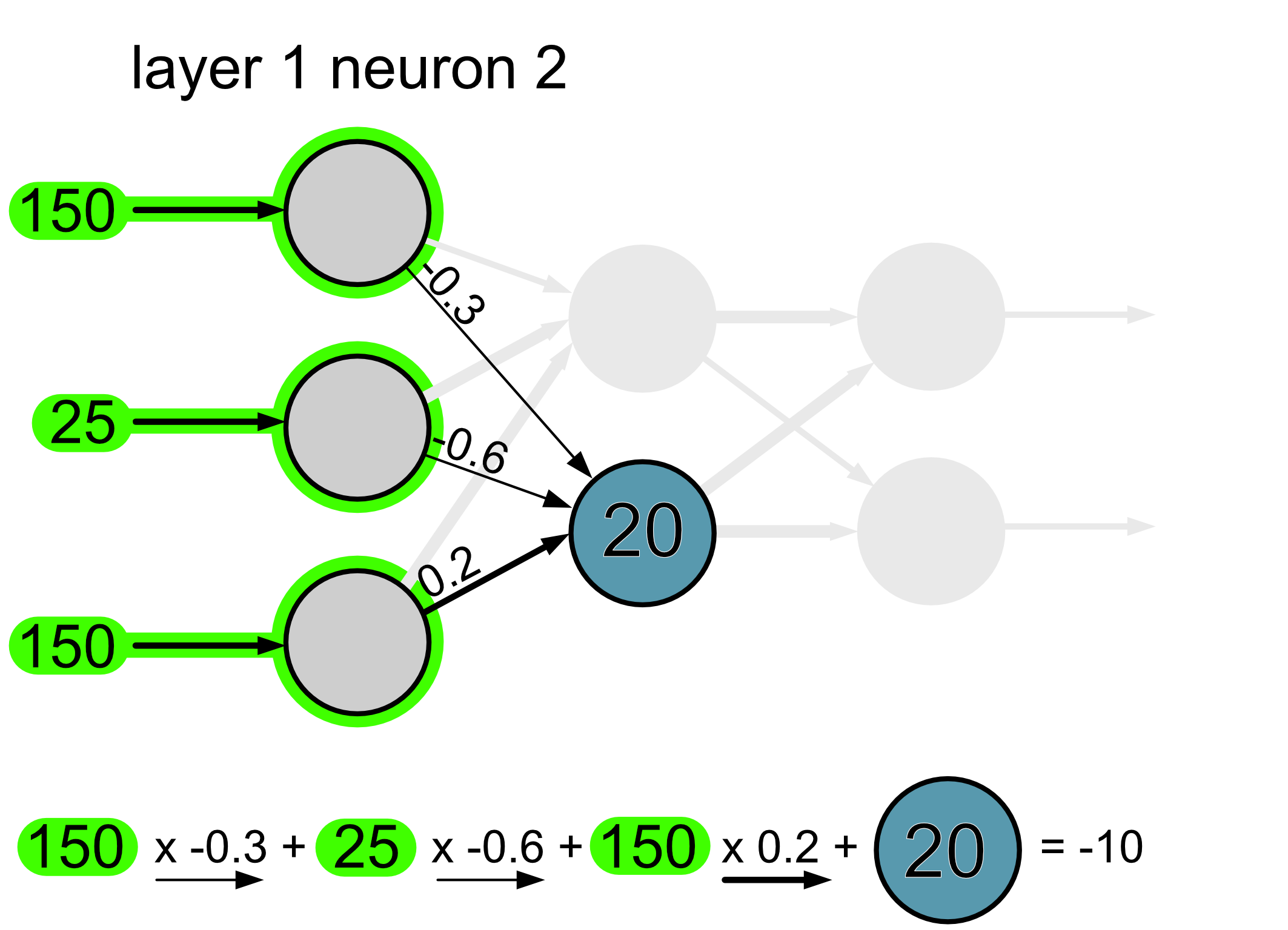
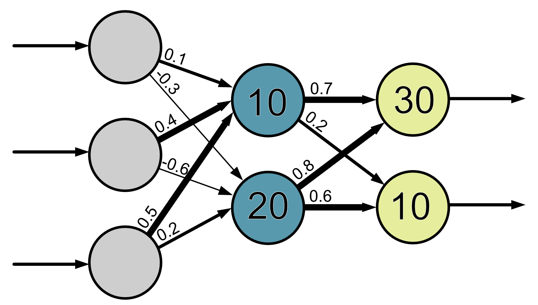
Here is a visual of how the information has flowed through thus far.
The next step is to apply something called an activation function. One of the most commonly used functions is called a ReLU function. It looks like this:
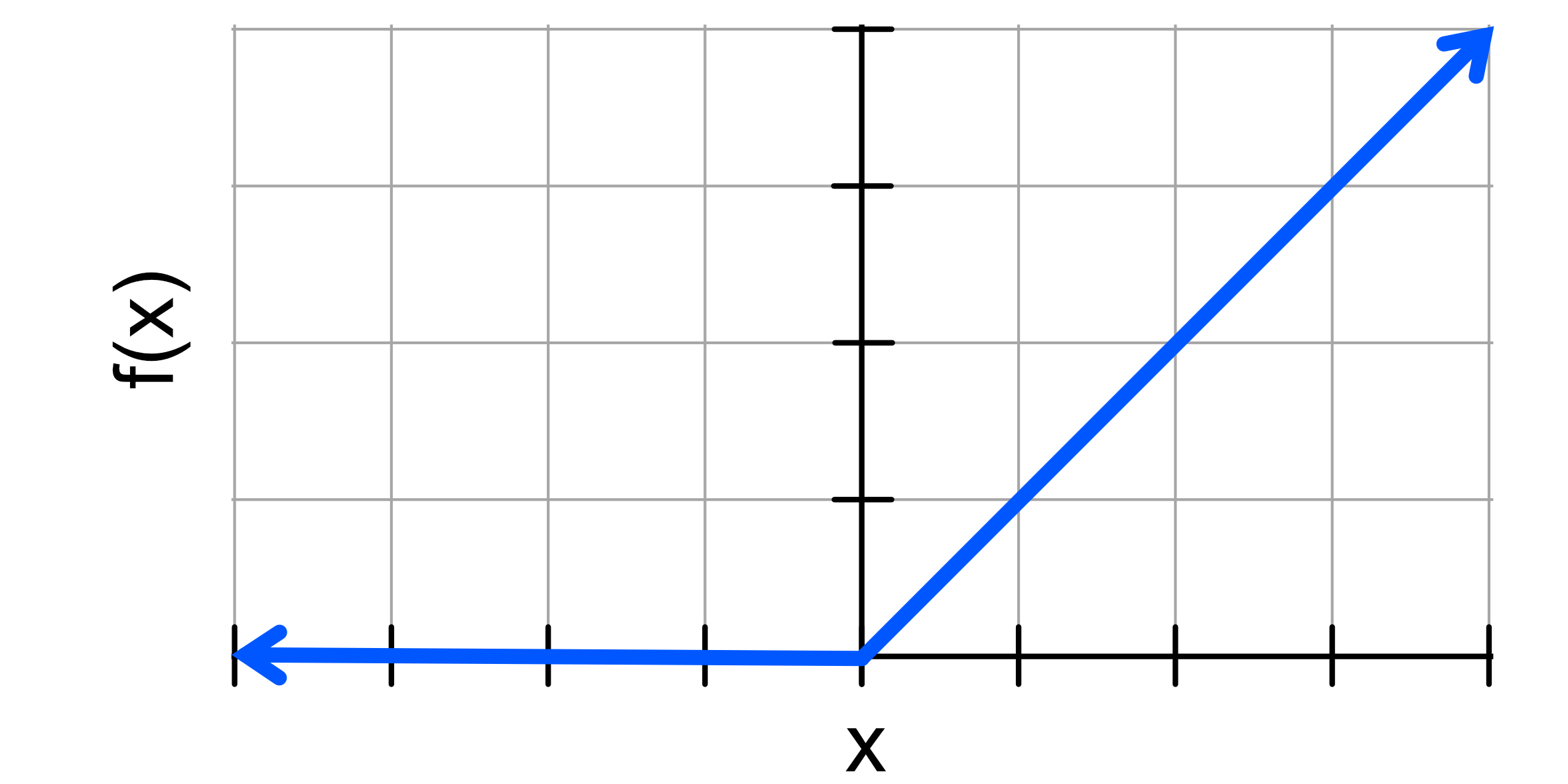
When we apply these to the neuron outputs we just calculated we find f(110) = 110 and f(-10) = 0.
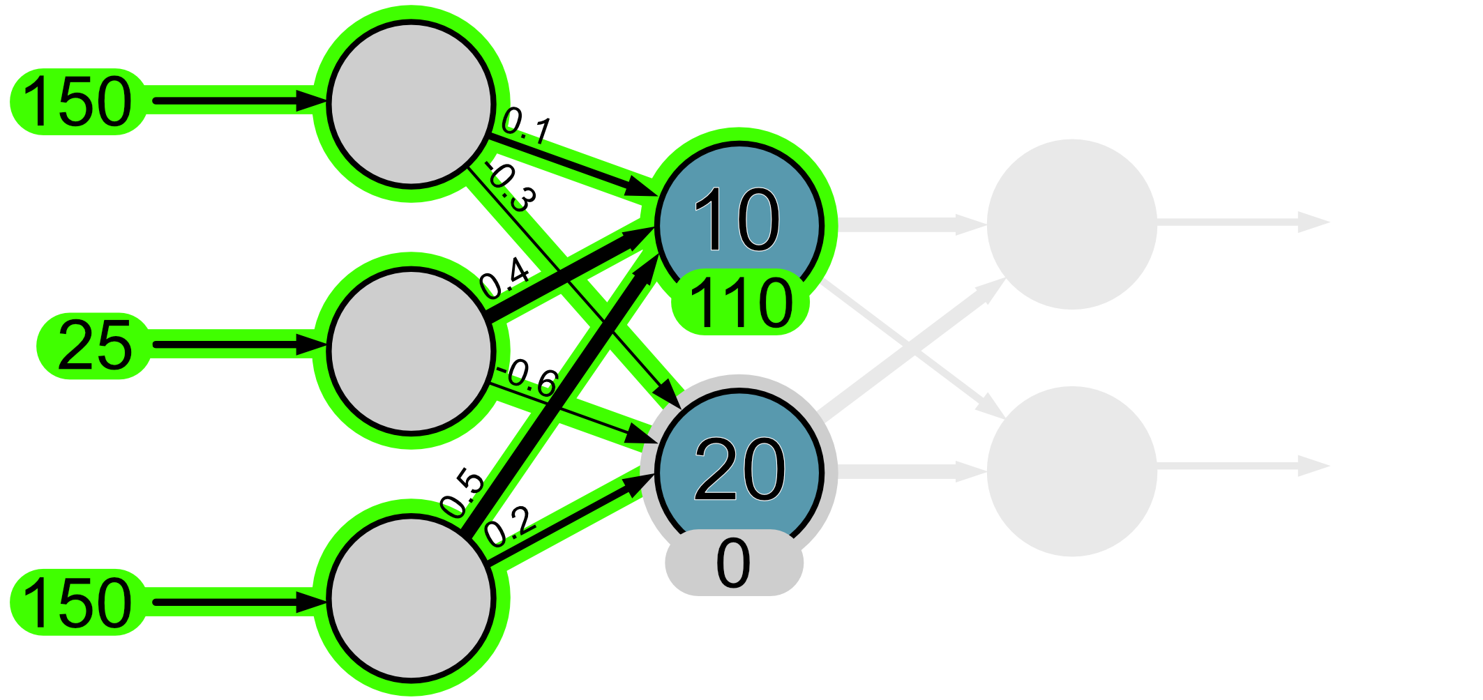
What you’ll have noticed is that the output of neuron 2 is set to 0. This is analogous to a neuron that has been activated, i.e. it hasn’t ‘fired’.
When your brain is active the neurons emit pulses, which we often refer to as ‘firing’. You might have heard this figuratively for example,”That idea really got my neurons firing” or “I had too much caffeine and I can my neurons firing off like crazy!”

So what the ReLU activation function does is that it requires a neuron’s output to be greater than 0, otherwise the neuron isn’t considered active and doesn’t continue to propagate information. You’ll notice here that the bias plays an important role in this calculation. The larger the bias is, the greater the tendency for that neuron to fire.
In regression, the activation function is typically only applied to neurons in the hidden layer, we do not apply it to neuron outputs in the output layer. We’ll see later when we get to classification that sometimes functions are applied to the output layer.
Let’s continue now with the rest of our network.
Again, to make things easier we’ll look at each neuron separately.
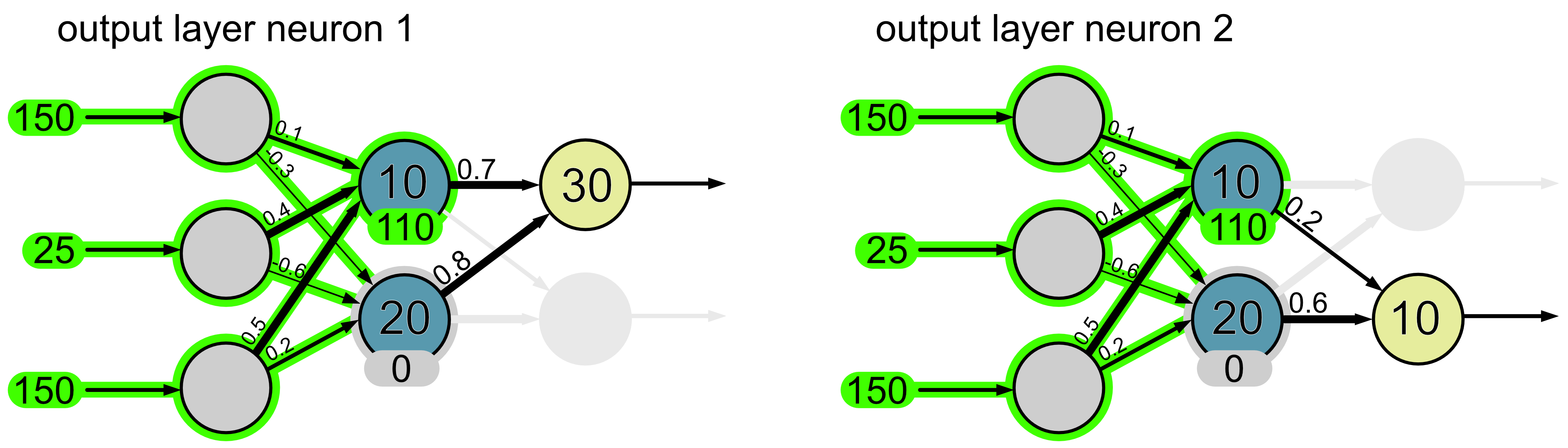
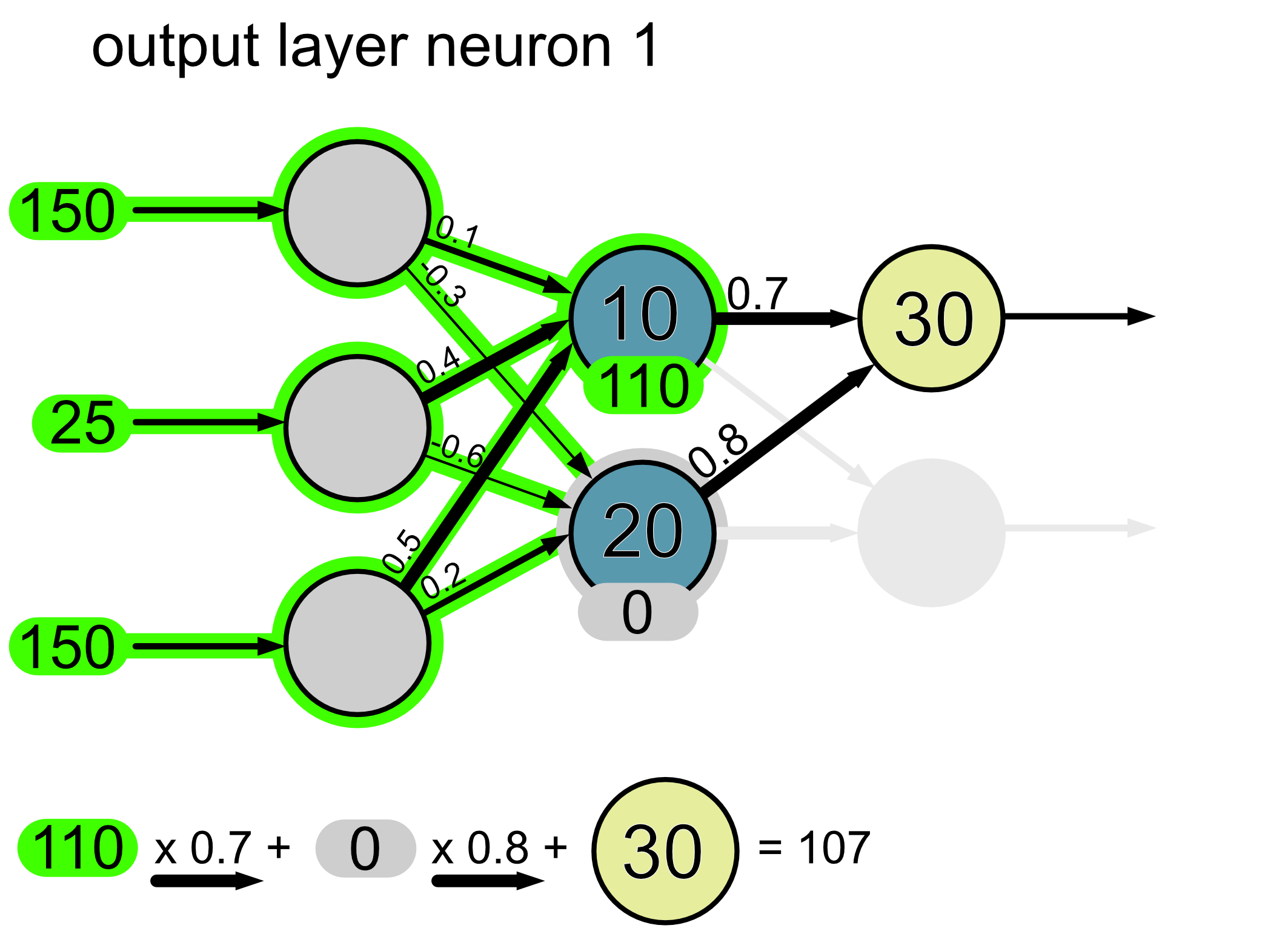
Here’s the calculation for neuron 1.
Here’s the calculation for neuron 2.
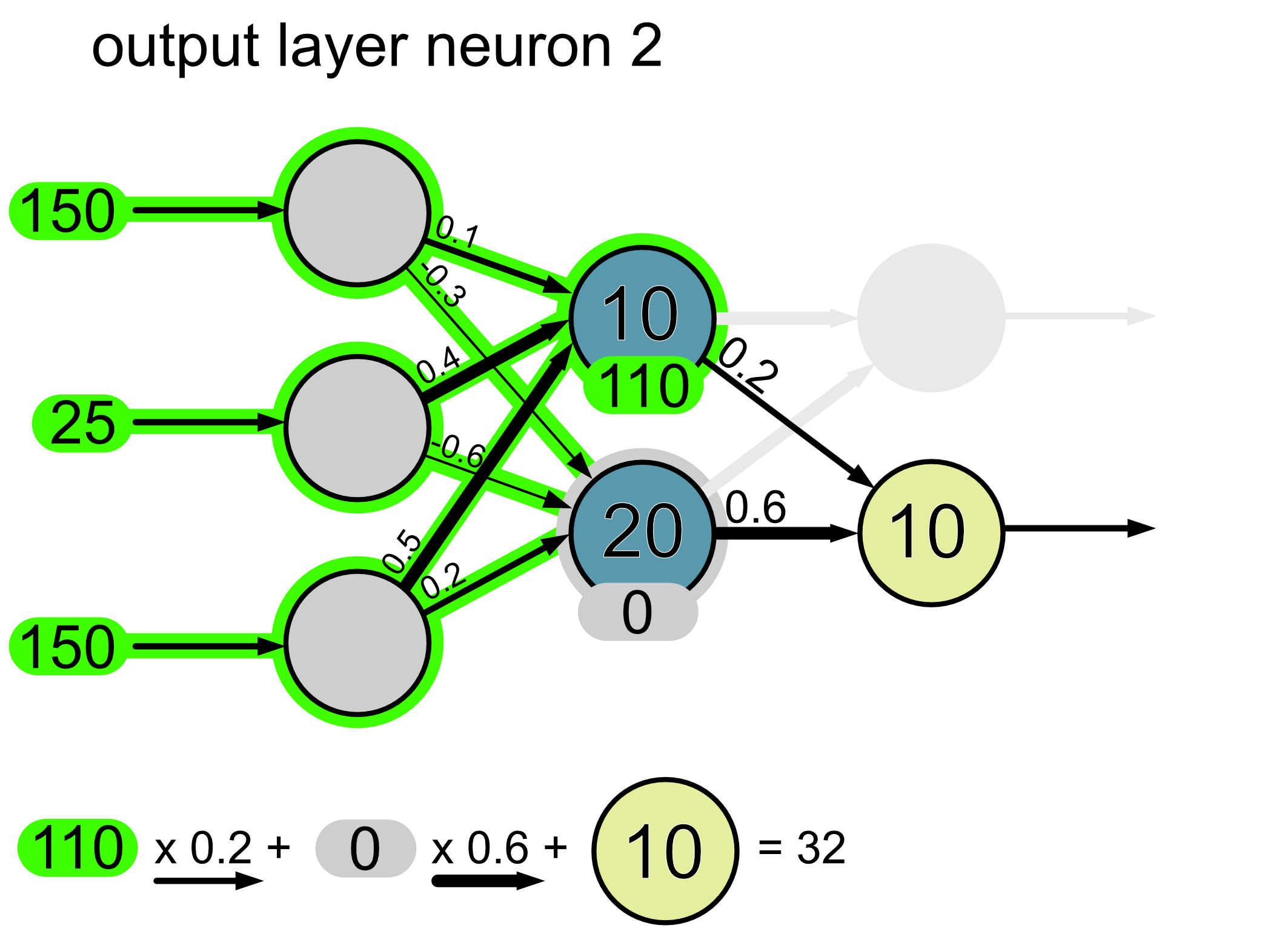
Since this is an output layer, we do not apply an activation function. Thus the final output of our network is a hue of 107 and a saturation of 32.