2.6. Logistic Regression#
Logistic regression is a form of supervised learning (data is labelled) used for binary classification. Binary, meaning ‘two’, means that in binary classification the goal is to assign each sample to one of two classes.
Examples of binary classification problems include:
Identifying whether a picture is of a cat or a dog
Determining if a patient has covid, or does not have covid
Predicting with a student will pass or fail an exam

Consider the following dataset:
Time Spent Studying (hours) |
Exam (Fail 0/Pass 1) |
|---|---|
4.5 |
1 |
8 |
1 |
1.5 |
0 |
3.5 |
1 |
5.5 |
1 |
3 |
0 |
6.5 |
1 |
We can plot this data out on a graph as shown below:
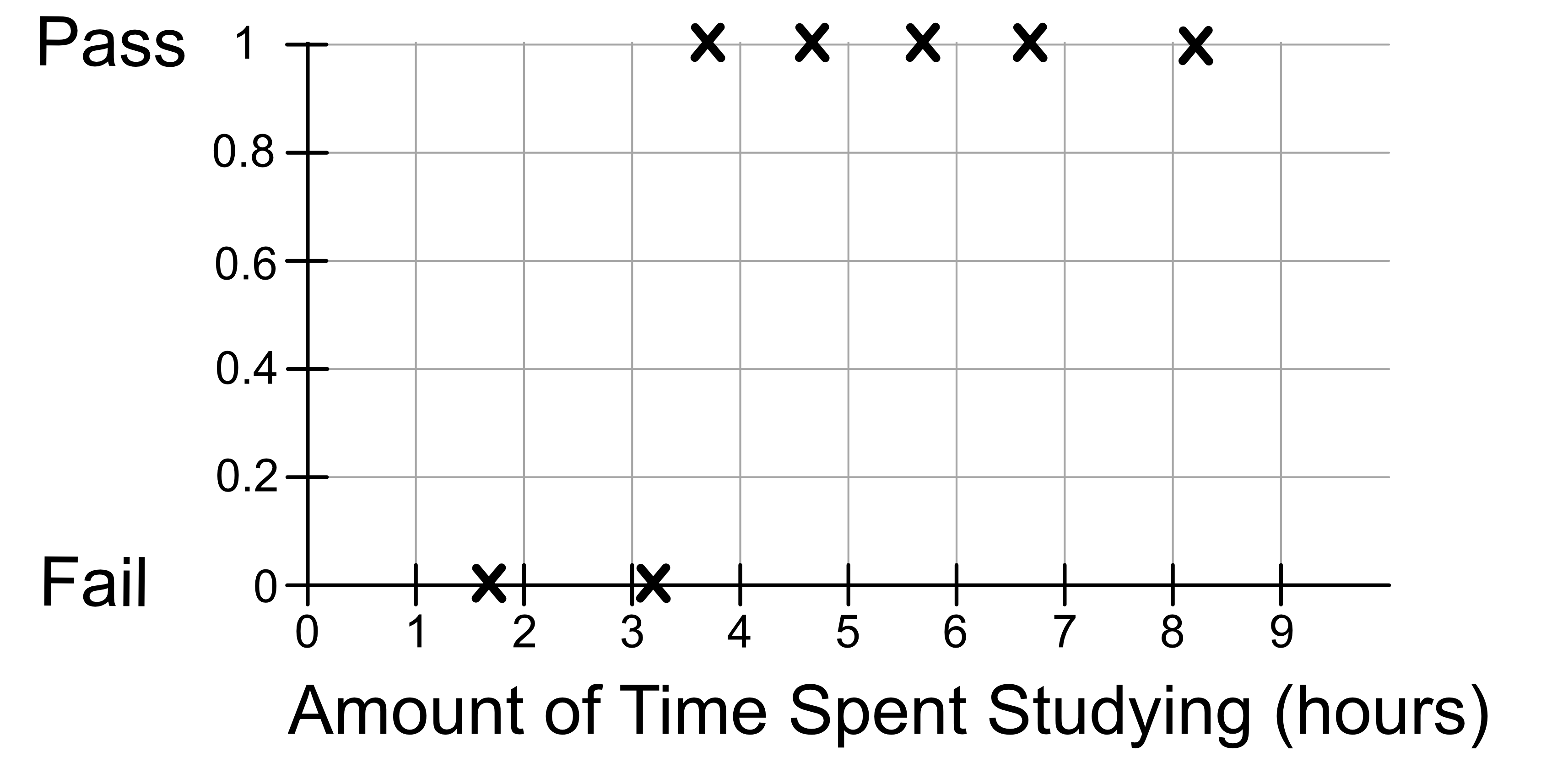
Notice that all of the y values of the data are either 0 or 1. To fit a curve to this data we use the logistic function. In logistic regression, the model can be described by the following mathematical equation:
If we were to fit a logistic function to our data, it would look something like this:
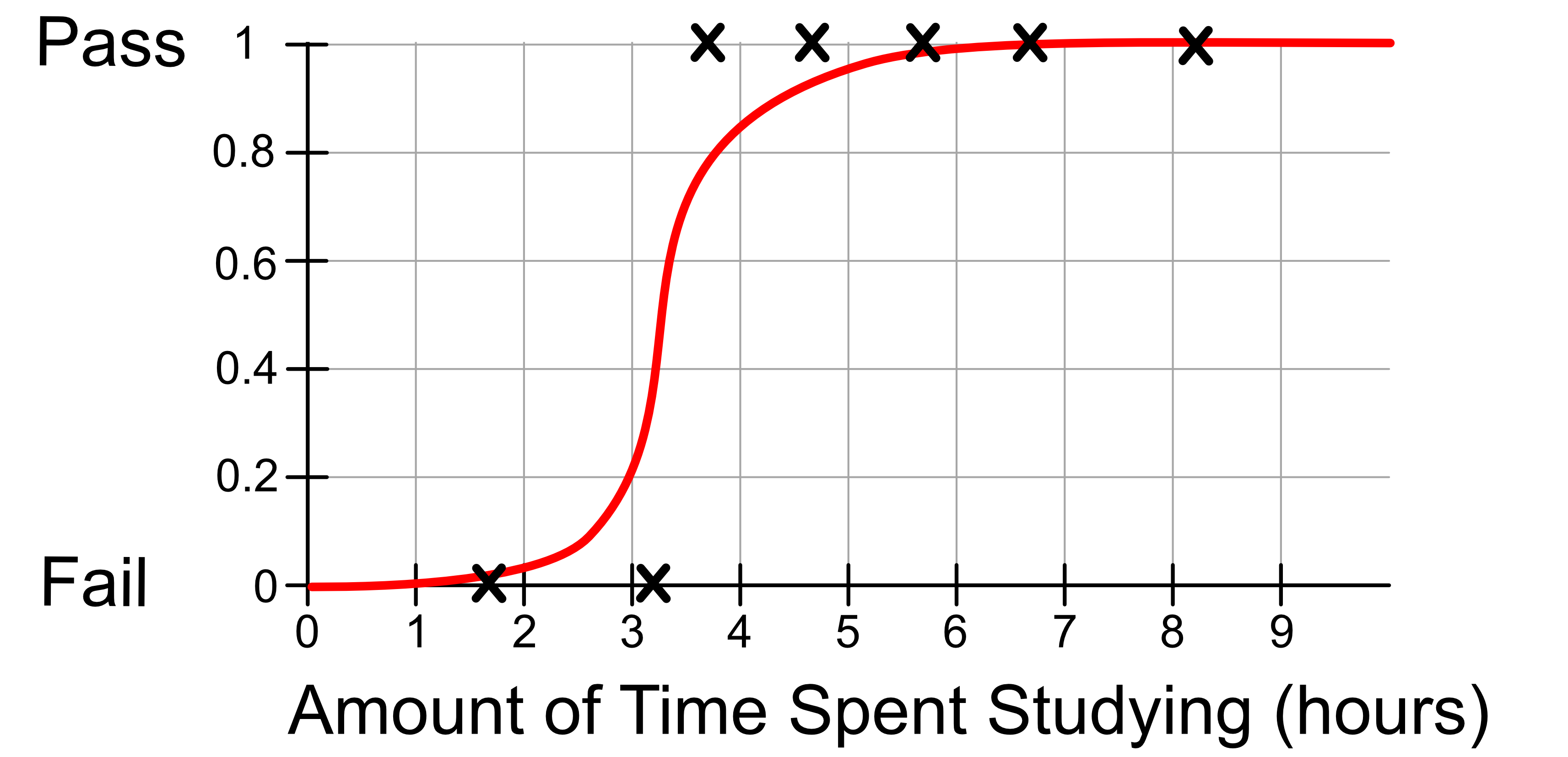
The logistic function will actually predict a number between 0 and 1, which we interpret as a probability of the sample belonging to class 1.
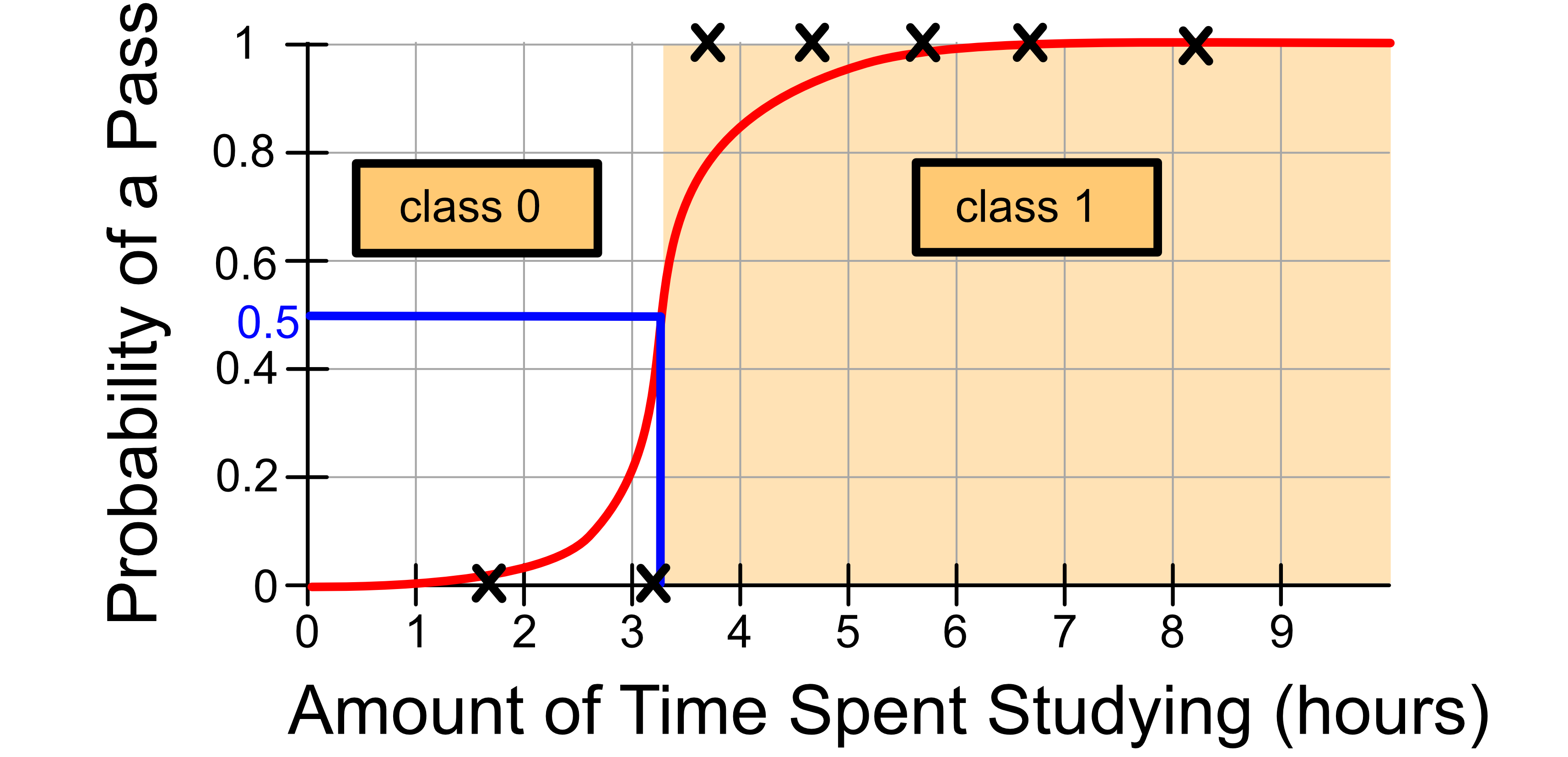
If this probability is over 0.5, then we assign the sample to class 1
If the probability is under 0.5, then we assign the sample to class 0
This means if we look at where the model crosses above a probability of 0.5 the model will always predict class 1 and below that the model will always predict class 0.
In our example, the logistic regression model predicts that a student will pass the exam if the spent at least 3.1 hours studying.
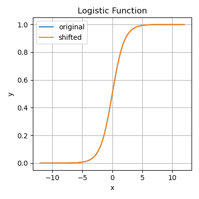
You can change the shape of the function by changing \(\beta_0\) and \(beta_1\).
\(\beta_0\) will shift the curve horizontally. The vertical part of the curve will sit at \(-\beta_0\).0
The sign of \(\beta_1\) (i.e. if \(\beta_1\) is positive or negative) changes the way the function ‘faces’.
The value of \(\beta_1\) will change how steep the vertical part of the curve is. The large the value, the steeper the curve.
You can experiment with changing the values of \(\beta_0\) and \(\beta_1\) in the code below.
import matplotlib.pyplot as plt
import numpy as np

beta0 = 0
beta1 = 1

x = np.linspace(-12, 12, 200)
y = 1 / (1 + np.exp(-x))  # original function where beta0 = 0 and beta1 = 1
yshift = 1 / (1 + np.exp(-(beta0 + beta1 * x)))

plt.figure(figsize=(4, 4))

plt.plot(x, y, label="original")
plt.plot(x, yshift, label="shifted")
plt.xlabel("x")
plt.ylabel("y")
plt.title("Logistic Function")
plt.grid()
plt.legend()
plt.tight_layout()
plt.savefig("plot.png")
Output
2.6.1. Glossary#
- Logistic regression#
A supervised learning algorithm used for binary classification that predicts a probability using a logistic function.
- Binary classification#
A classification task where each sample is assigned to one of two classes.
- Logistic function#
A function used in logistic regression that outputs a value between 0 and 1, interpreted as a probability.